Smartsheet: Cross Sheet References (X-Sheet Ref) are here. Now what?
It has been a long time coming. I wasn’t sure if it would. I wasn’t sure if it should. But it is here, so we better get ready.
(Warning: Personally, I’m not fully ready yet. Every time I look at a Sheet or Report, my mind spins with redesign possibilities. Or maybe it’s the meds. I’m fighting a bad cold, allergies, or a mild case of the flu as I write this. I’m pretty sure this post will evolve.)
It
So, what is it? It is cross sheet references in Smartsheet. I’ll call them X-Sheet Refs here (I doubt anyone will confuse them with exposure sheets).
Smartsheet in the Before Times (pre-2018-02-06) could not easily have something like this:
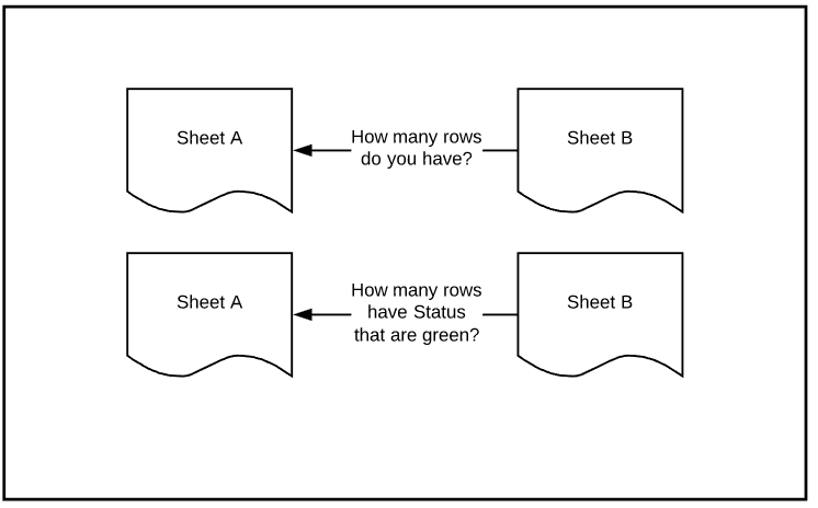
where Sheet B would like to query Sheet A for how many rows it has, or how many [Status]’s are green. Instead, Sheet A would need to be setup to get that information itself and the results of that would passed to Sheet B using Cell-Linking.
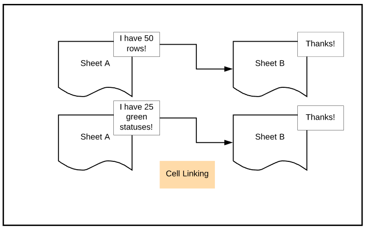
The end result of this was that many sheets had some portion of it devoted to “Summary Sections” or “KPI Sections”. The names vary, but the idea was the same. Somewhere outside the normal user-visible rows and columns, the important stuff was consolidated, summed, counted, averaged, weighted, and so on.

Those sections could be at the top, at either side (left or right of the user visible area), or at the bottom.
X-Sheet Refs will change that. Sometimes.
But Wait, What About VLOOKUP?
You may have seen this:
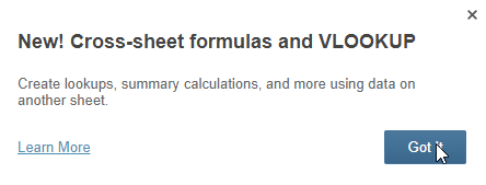
Isn’t VLOOKUP the best part?
No. We already had the ability to use LOOKUP across sheets. LOOKUP takes (took) input {what am I searching for?} and results in an output {here’s what I found}. It does this search on a range of cells . I wrote this post about Nested-IF‘s that uses a LOOKUP table on a different sheet to get its results. As far as I can confirm (I discussed with people who know), there is NO CHANGE to the LOOKUP() function, except for the name change. What is changed is that it will EASIER to perform the referencing. Whereas before, each cell or contiguous range of cells were linked from one sheet to another. Now, we’ll set up a X-Sheet Ref and just use it again and again, on the same sheet (we’ll come back to that and why it in italics.)
Now I’m confused, what did we get?
Let’s go back here:
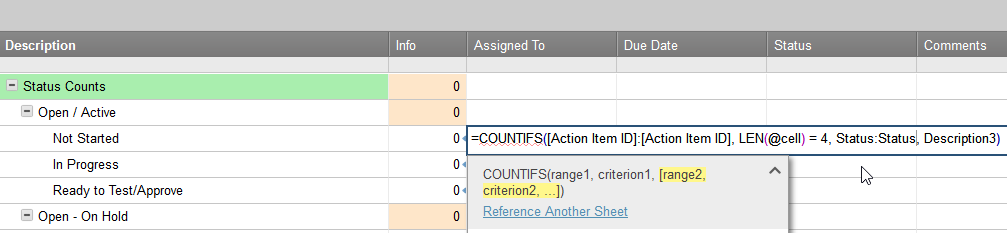
In the Before Times, I would build a formula that looked something like this:
The cell that had the formula would then be linked out to another Sheet, shown on a Dashboard, or be part of Report.
Now, we can instead move the calculation to Sheet B and reference back to Sheet A.
By moving the formula to Sheet B, we’ll be able to (not a complete list! See ‘mind spinning’ above)
- Cleanup Sheet A – less rows and/or columns. Better performance
- When performing calculations on a whole column, you won’t need to have an additional location for the cell (to avoid circular references)
- The Summary Sheet / Roll-Up Sheet / KPI sheet (Sheet B) can have the same column names and types as where the data resides on Sheet A, so careful design of Reports can show both the overview (Sheet B) and the details (Sheet A) together
- When Sheet A is very dynamic, less rigor will be necessary to deal with row addition and deletion. I think, I’m still testing this concept and may be for some time.
So are you excited or not?
Very. But.
I’ve seen people asking for something it isn’t. This does not turn Smartsheet into a database. Sorry to break the bad news.
Going back to that Nested-IF example, some people use this formula to return the text name for a month based on its number:
IF(MONTH([Start Date]2) = 12, “December”, IF(MONTH([Start Date]2) = 11, “November”, IF(MONTH([Start Date]2) = 10, “October”, IF(MONTH([Start Date]2) = 9, “September”, IF(MONTH([Start Date]2) = 8, “August”, IF(MONTH([Start Date]2) = 7, “July”, IF(MONTH([Start Date]2) = 6, “June”, IF(MONTH([Start Date]2) = 5, “May”, IF(MONTH([Start Date]2) = 4, “April”, IF(MONTH([Start Date]2) = 3, “March”, IF(MONTH([Start Date]2) = 2, “February”, IF(MONTH([Start Date]2) = 1, “January”, “N/A”))))))))))))
Ich.
What I have long done is somewhere on a Sheet needing this functionality, I add a table.
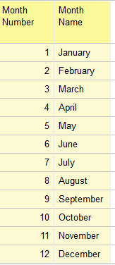 And then get my Month Text like so:
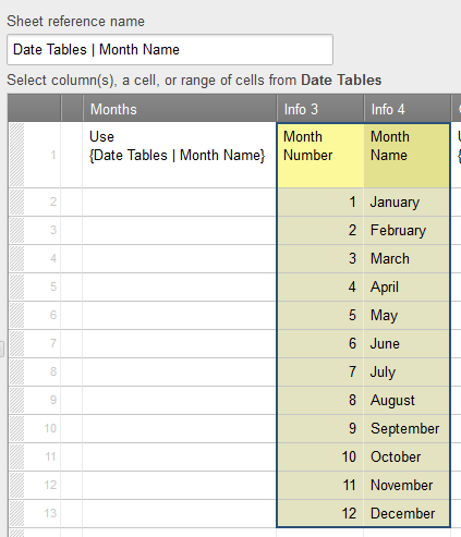
=LOOKUP(MONTH([Start Date]2), [Info 3]1:[Info 4]13, 2, false)
where [Info 3] and [Info 4] are columns created just to hold the data. (New syntax will be VLOOKUP())
Now, just as we can reference a whole column, we can reference just part of the sheet too.
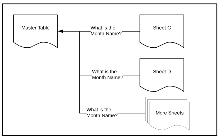
Once I move my table data to a Master Sheet, I would like to be able to reference it from any sheet.
And I can.
The problem is that the X-Sheet Ref NAME is created and maintained on the DESTINATION SHEETS. That is Sheet C and Sheet D and all of other sheets will create a reference to the Master Table sheet. Sheet C could call the table {My Month Text Table} and Sheet D could call it {Date Tables | Month Name} and the rest could call it whatever they like: {Bob}, {MT}, or anything else.
We won’t (yet) be able to Copy the X-Sheet Ref from Sheet C to Sheet D. If we make a copy of Sheet C, the reference will go with it, but just not to existing sheets.
For me, if it was only about lookup tables, then that’s where using the X-Sheet References falls short. When using it for LOOKUPs / VLOOKUPs, it does help that I can build a reference to the entire table, once, and use it throughout my Sheet. But the rest, not so much.
Enough about VLOOKUP
Almost done. Not that long ago (2016-08-06 to be exact), Smartsheet released the LOOKUP function. Some people went nuts because it wasn’t the VLOOKUP they grew up with in Excel. At the time, I wrote a defense of the design choice, but never got around to finishing it. Buried in that writing was what I wanted (and still want)
I want to be able to reference tables. Not Sheets, but just tables.
I should be able to define the columns and add data to the cells in each row.
I don’t need (but may want later) formatting and conditional formatting and notifications and reminders and to see the data in a Card View or Gantt chart … but I really just want to be able to maintain the data in the same place and then tell the users that need to know how to get the data into their sheet.
I didn’t get that. I got something different. I think maybe I got something better and it has nothing to do with tables.
A Whole New World
Nearly every one of the Sheets I have looked in the last 6 days since the release could use some tweaking or even major redesigns.
I rebuilt a few already. It takes a little bit of time, but not as much as I expected. I’ve been bench marking the time to make the changes. Don’t fix what ain’t broke, but the interface I’ve ended up with more often than not has been cleaner and easier to maintain later. Again, I think. It has only been six days.
Here’s some things I know will help:
- Determine a Naming Convention that works for you. Stick to it. I haven’t fully committed to mine yet, but it will likely be something that contains the Sheet Name and a Description of the Range. I say ‘likely’ because I’m not overly fond of the results of the Save as New operation on the reference name when dealing with Workspaces.. I know there is one (or more) naming conventions that will work.
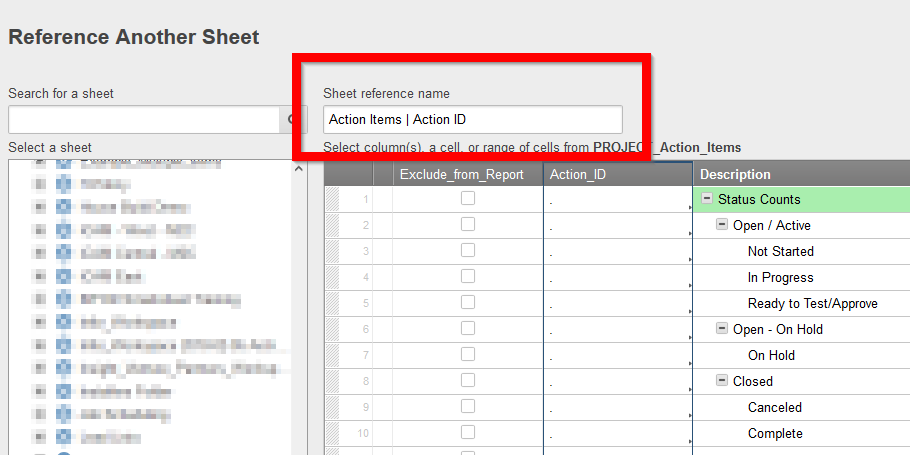
- Document them. I’ve been experimenting with either Sheet level Comments and/or Screen Shots of the Reference Another Sheet dialog. Find something that works for you.
- Where possible, use the same reference names for the same data set. That means there needs to be somewhere that you track the reference names and content outside of the Destination Sheets too.
- Keep the direction of data flow in mind. The flow is from the Source Sheet to the Destination Sheet, but it is the Destination Sheet that has the control. And their roles can be reversed. What does the Destination Sheet need and where is that data located.
I’m sure will pop up as I work with X-Sheet Refs more.
Final Thoughts
I’m fairly confident these aren’t my last words on the subject. There are areas of the possibilities I’ve only started to explore. I’ll be watching the Community for examples of where others are going. That’s where I get a lot of my inspiration.
If you like this post, please “Like” it. Every time my post gets liked, a fairy gets her wings. Or I’m more likely to post another one. It is one of those two, I’m sure.
If you are new to Smartsheet and want to check it out, click here. If you have questions about this post, add them below. If you have questions about something else in Smartsheet, post on the Community. I occasionally stop by to answer them and so do a lot of other talented people.
Comments