Finding “Next” Task in Smartsheet

Today I was trying to get some energy and motivation by perusing the  Smartsheet Community and I ran across a question that helped with those.

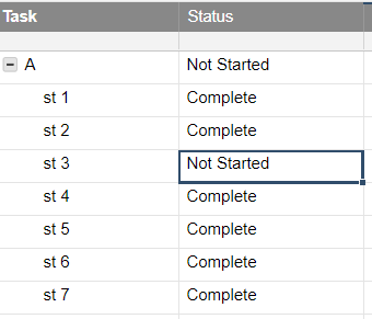
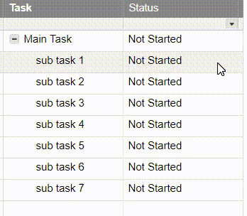
I will paraphrase the problem: A main task has a series of sub-tasks. The user want to check the status of each sub-task and return the status of the first non-completed task as the status of the whole/main task. While this rings a few alarm bells for my PM side, this wasn’t a customer and I didn’t want to dig into why this functionality was the use-case, rather the stated problem itself was interesting on its own. Add to this that another Community Member had taken a shot at the answer and his solution needed some changes.

Many times, the first response to these kinds of problems has some sort of Nested IF functionality as part or all of the solution. I could see at a glance that probably wasn’t going to work here because it wouldn’t be scalable. Based on other work I have been involved with recently, scalability is often on my mind, which helped get my head in the right spot to see the solution.

MATCH

The core of the solution lies in the MATCH function. Because we are dealing with a hierarchy, there’s a ready built range to deal with.

=MATCH(“In Progress”, CHILDREN(), 0)

will search an unsorted list (the children), looking for “In Progress”. If “In Progress” is found, it will return the row (based on the rows in the children) where it found it.

If it does not find “In Progress”, it will return an error, so let’s catch that with IFERROR. The error it returns is #NO MATCH, but any error will do for now.

=IFERROR(MATCH(“In Progress”, CHILDREN(), 0), 5001)

If there is an error thrown, I return 5001  for each unmatched type because that is beyond the (current) Smartsheet row limit and won’t be returned by a valid match, but I want it to return a number. I’m jumping ahead here, but for this particular formula when 5001 is returned, this is either because:

a. All children are complete

b. Some children are mis-typed (data validation might be recommended here)

c. I don’t search for blanks (but could based on recent changes to the MATCH function)

There’s one more reason why I use 5001 here, but I’ll get to that below.

The MATCH function will return a number for the first one it finds if it finds a match and the IFERROR will return 5001 if it is does not.

MIN

Next, for each of the non-Complete statuses, there is an associated IFERROR(MATCH()) and I find out which one is the smallest number (earliest in the task list) using the MIN function.

=MIN(IFERROR(MATCH(“Cancelled”, CHILDREN(), 0), 5001), IFERROR(MATCH(“In Progress”, CHILDREN(), 0), 5001), IFERROR(MATCH(“Not Started”, CHILDREN(), 0), 5001), IFERROR(MATCH(“Waiting”, CHILDREN(), 0), 5001))

Again, if none are found, the minimum will be 5001. If any are found, we’ll have the row number of the list.

INDEX

That row number is a perfect fit for INDEX. 

=INDEX(CHILDREN(), MIN(…))

This returns the sub-task’s status that was found by MIN. We could also use another range here to return something else – say the Start Date or the Task Name of the “Next” one, but for this example, we’ll just return the status.

This brings us back to that 5001 again.  5001 is an invalid input to the INDEX() function, which throws an error. If we get 5001, then we didn’t find anything else.

“Eliminate all other factors, and the one which remains must be the truth.”
Arthur Conan Doyle (as Sherlock Holmes)

Wrapping the INDEX() up in another IFERROR, and we return “Complete” when we have an error (see a and b) above.

=IFERROR(INDEX(CHILDREN(), MIN(IFERROR(MATCH(“Cancelled”, CHILDREN(), 0), 5001), IFERROR(MATCH(“In Progress”, CHILDREN(), 0), 5001), IFERROR(MATCH(“Not Started”, CHILDREN(), 0), 5001), IFERROR(MATCH(“Waiting”, CHILDREN(), 0), 5001))), “Complete”)

This may, unfortunately, mask a different error, and to be honest, I’m not completely comfortable with that, but to fix it (I think) would require something that I would be even less comfortable with.

There might be a way to make this formula more compact but I have a solution so I’ll leave it alone (for now).

Final Thoughts

As I mentioned at the beginning, this functionality sets off warning bells if I were the PM, but there are enough edge cases and special circumstances that this may be exactly what is needed. In addition, I can think of a few instances where the formula can be modified to provide a different (perhaps better) solution than what I was using before. And that can’t be a bad thing.

If you like this post, please “Like” it. Every time my post gets liked, a monkey gets a banana. Or I’m more likely to post another one. It is one of those two, I’m sure.

If you are new to Smartsheet and want to check it out, click here. If you have questions about this post, add them below. If you have questions about something else in Smartsheet, post on the Community. I occasionally stop by to answer them and so do a lot of other talented people.